 This second article in a three-part series on gas laws describes how to use a Mason jar to collect data and demonstrate the pressure-temperature relationship, Gay-Lussac’s law. Its huge advantage is that the gas temperature is measured, NOT the temperature of the water bath.
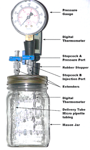
In this lab, a Mason jar lid has three holes, each with an attachment — a digital thermometer, a pressure gauge with a stopcock (A) and an injection port with a stopcock (B). The one shown (Fig. 1) was purchased1 but a teacher could also build this apparatus. The difficult part is creating a seal around the attachments when they are inserted into the holes.
To prepare the Mason jar, remove the pressure gauge along with stopcock (A). Using the gas distribution apparatus,2 add gas into injection port (B) by either the upward or downward displacement of air. Appropriate gases are nitrogen, oxygen, carbon dioxide, methane and propane. Reattach the pressure gauge and close both stopcocks. Open the injection port (B) and use a 60 mL syringe to inject an additional 60 mL of the gas. After the Mason jar is placed in an ice bath, this 60 mL of additional gas avoids the pressure gauge needle going below zero — the gauge does not read below zero. The gauge is similar to a tire gauge. It measures the pressure above atmospheric pressure, not the absolute pressure. Initially a small pressure should be recorded on the pressure gauge. The pressure is read at the corresponding temperature by opening and then closing stopcock (A). This method allows students the time to record a “static” pressure — without the pressure reading changing while measuring.
| Temp | Total p | Heat gauge p | Cool gauge p | Average p |
| (± 0.2 oC) | (± 1 kPa) | (± 0.5 kPa) | (± 0.5 kPa) | (± 0.5 kPa) |
| 10 | 105.7 | 6.0 | 6.0 | 6.0 |
| 15 | 106.7 | 7.0 | 7.0 | 7.0 |
| 20 | 107.5 | 8.0 | 7.5 | 7.8 |
| 25 | 109.0 | 9.0 | 9.5 | 9.3 |
| 30 | 110.2 | 10.5 | 10.5 | 10.5 |
| 35 | 113.0 | 12.5 | 14.0 | 13.3 |
| 40 | 115.5 | 16.0 | 15.5 | 15.8 |
| 45 | 117.0 | 17.0 | 17.5 | 17.3 |
| 50 | 119.0 | 19.0 | 19.5 | 19.3 |
| 55 | 120.5 | 20.5 | 21.0 | 20.8 |
| 60 | 121.0 | 21.5 | 21.0 | 21.3 |
| 65 | 124.7 | 26.0 | 24.0 | 25.0 |
| 70 | 126.2 | 27.5 | 25.5 | 26.5 |
| 75 | 127.5 | 29.0 | 26.5 | 27.8 |
| 80 | 129.2 | 31.0 | 28.0 | 29.5 |
| 85 | 131.2 | 32.0 | 31.0 | 31.5 |
| 90 | 133.7 | 34.0 | 34.0 | 34.0 |
- Atm pressure 99.7 (± 0.5) kPa
To start the experiment, the Mason jar is placed in an ice-water bath until the temperature of the gas has fallen just below 10 oC. A hot plate is then used to warm the water bath. Take readings of temperature and pressure every 5 oC starting with 10 oC and going to 90 oC. (measured as the heat gauge pressure). Cool the water bath using ice and repeat the pressure reading every 5 oC from 90 oC to 10 oC (measured as the cool gauge pressure). A typical set of data is shown for air (Fig. 2). The measured gauge pressure is added to atmospheric pressure to determine the total pressure.
A plot of total p vs T yields a straight line, which passes through the temperature axis within less than 10% of absolute zero, as shown (Fig. 3). Encourage students to add another temperature axis below the Celsius axis and then to draw another pressure axis starting at the Celsius intercept. Have the students create a new temperature scale with zero at the intercept — I use “E” for the “Eix” scale. Label the new temperature axis using his or her surname to honour their creating this new temperature scale. Determine how the new temperature scale relates to the Celsius scale. Discuss the implications of such a scale and why it is a theoretical scale while Celsius is an empirical scale. This is your opportunity to introduce the Kelvin scale.
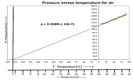
Fig. 3. Pressure vs temperature graph of air.
Notes:
- The apparatus is available at S17 Science (EQ 888 S17 Science Gas Kit: $90 US or CAN $108.00). Other gas equipment kits can also be purchased. See www.s17science.com.
- A different way to do gas laws — Part 1: Pressure-volume relationship, Chem 13 News, September 2015